
The recent rise in interest rates has, among other things, led to dramatically lowered transaction volumes which, in turn, has led to much uncertainty about today’s market-clearing capitalization rates – as well as where such rates will come to rest in the future.
This note addresses two aspects of the uncertainty surrounding (current and future) cap rates; in particular, the non-linear relationship between prices and cap rates leads to: 1) price convexity and 2) skewed v. symmetrical volatility estimates.
PRICE CONVEXITY
Like other income-generating assets, commercial property prices reflect “convexity” with regard to changes in cap rates (just as fixed-income prices reflect convexity with regard to changes in interest rates).1
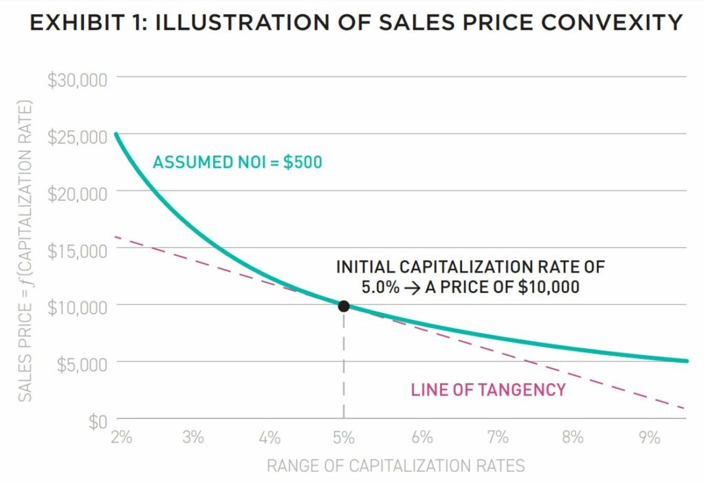
As illustrated in Exhibit 1, convexity implies that the dollar change in property values is greater for a given basis-point change in cap rates when cap rates are low and, conversely, the dollar change in property values is lesser for a given basis-point change occurs when cap rates are high.
In other words, the relationship between the dollar value of price changes is non-linear (and convex) with regard to the basis-point change in cap rates.2 For purposes of illustration, let’s assume certain real estate investors (and lenders) are either: estimating today’s market-clearing cap rate to equal 5%, or forecasting an ending (or reversionary) cap rate of 5%.3 In either case (depending on the investor’s objectives), let’s assume net operating income (NOI) of $500 so that the property’s price (today or in the future) equals $10,000:4
Let’s revisit this simple illustration of price convexity by considering a 100 basis-point change in the cap rate, from the assumed starting point of a 5% initial cap rate, as shown in Exhibit 2.
As indicated in Exhibit 2, decreasing the initial cap rate by 100 basis points results in an ending cap rate of 4% and an increase in the sales price to $12,500, for an increase of 25% from initial estimate of $10,000.
Meanwhile, increasing the initial cap rate by 100 basis points results in an ending cap rate of 6% and a decrease in the sales price to approximately $8,333, for a decrease of approximately 16.7%.
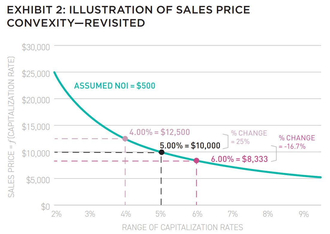
This difference (i.e., 25% v. -16.7%) illustrates the convexity in real estate prices for a given change in cap rates. Said another way, convexity implies that the percentage change in price varies with a constant change (measured in basis points) in cap rates.
Given today’s conversations about the potential increases in interest rates and cap rates, the convexity in real estate prices suggests that the fall (measured by the percentage change) in prices due to rising cap rates is less than the earlier benefits associated with heretofore falling cap rates. This is, of course, “cold comfort” to investors (and lenders).
SKEWED V. SYMMETRICAL VOLATILITY ESTIMATES
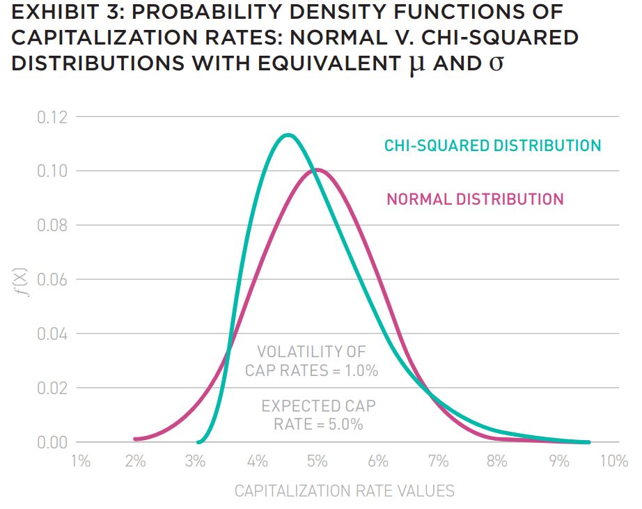
The importance of convexity is also highlighted when we consider the distribution of potential (current and/or reversionary) cap rates. As suggested earlier, such distributions may not be normally distributed. So as an illustration, let’s compare the hypothetical in which the distribution of cap rates is modeled by the symmetrical normal distribution and by the asymmetrical chi-squared (or χ2 ) distribution, where both distributions5 have the same expected value and the same volatility: µ = 5% and σ = 1% (these values were arbitrarily chosen – investors should select parameters consistent with their expectations), as shown in Exhibit 3:
Other asymmetrical distributions are, of course, possible and would also serve to help make the points below.6 While both distributions have (by design) the same first two moments (µ = 5% and σ = 1%), the chi-squared distribution displays positive skewness: fewer instances of extremely low cap rates and a mode of ≈4.5% (as compared to a mean of 5%). On the other hand, the normal distribution displays the familiar bell-shaped (symmetrical) distribution, but importantly includes greater instances of extremely low cap rates. It is these extremely low cap rates that produce correspondingly extremely high property prices. The two distributions’ far-right tails (i.e., high cap rates) ae similar, and therefore produce similar estimates of extremely low property prices.
Against this backdrop of price convexity and capitalization-rate dispersion, let’s consider the potential dispersion in (current and/ or reversionary) property values, as shown in Exhibit 4:
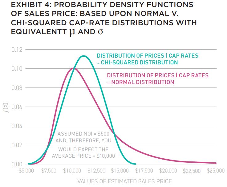
At first blush, it’s a bit surprising that the symmetrical distribution of cap rates (i.e., the normal distribution) produces the positively skewed distribution of prices (i.e., extremely high prices).7 Given today’s investment climate, the exceedingly high prices associated with the normal distribution seem unattainable.
Instead, it is the asymmetrical chi-squared (or χ2 ) distribution (i.e., with its fat right-tail) of cap rates that produces a near-symmetrical distribution of potential sale prices.
The interplay of price convexity and the assumed dispersion of cap rates also produces interesting first-two moments (µ and σ), under the two distributions, for estimated sales prices, as shown in Exhibit 5:
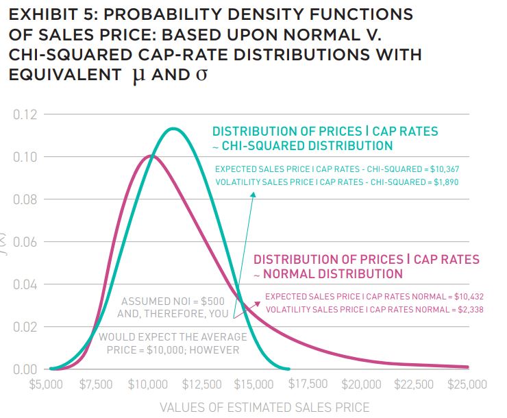
Consider the summary statistics for each distribution, starting with the expected values: the expected property price is approximately $10,432 under the normal distribution and $10,367 under the chi-squared distribution.
Note that the expected prices are higher than the estimated price ($10,000) assuming no uncertainty (or dispersion) in anticipated cap rates. The difference is due to the combination of price convexity and uncertainty. (This is another example of the adage associated with non-linear relationships: “The expectation of the average differs from the average expectation.”)
Additionally, the standard deviation of property prices is approximately $2,338 under the normal distribution, but only $1,890 under the chi-squared distribution; on a relative basis, the volatility of property prices is greater under the normal distribution (i.e., the coefficient of variation (σ/µ) ≈22.4% for the normal distribution and ≈18.2% for the χ2 distribution).
APPLICATIONS
Among many potential ramifications of the dynamics discussed here, consider four:
- the lender’s estimate of its collateral value (the non-recourse lender effectively provides the borrower with a put option),
- the developer’s estimate of land value is essentially a call option on the value of the future to-be- built project vis-à-vis the all-in costs of development,
- the levered equity investor essentially owns a call option on the property’s value relative to the loan balance, and
- the expected value of the general (or operating) partner’s carried interest is also a call option on the property’s future profitability.
The expected value of all such options depends on the volatility of the underlying asset. Investors (and lenders and modelers) beware!
EXLORE THE FULL ISSUE

ALSO IN THIS ISSUE
AFIRE INTERNATIONAL INVESTOR SURVEY: Q1 2023 PULSE REPORT
Gunnar Branson and Benjamin van Loon | AFIRE
VALUATION CHALLENGE: SOLVING THE CRISIS IN COMMERCIAL REAL ESTATE VALUATION
Matt Pomeroy, MAI and Jackie Bowie | Chatham Financial
CONVERSION CALCULATOR: LEGAL OR NOT, A DYNAMIC CITY WILL CONVERT UNUSED OFFICES
Jim Costello | MSCI Real Assets
UNDERWRITING ROADBLOCKS: CAN THE HOSPITALITY MODEL OF UNDERWRITING SAVE OFFICE VALUES?
Joshua Harris, PhD | Lakemont Group & Fordham University
VACANT SPACE: OFFICE-USING JOBS AND DEMAND INCONGRUITY
Stewart Rubin and Dakota Firenze | New York Life Real Estate Investors
HIKING TRAILS: SHOULD INVESTORS CONSIDER ALLOCATIONS TO FLOATING-RATE DEBT?
Dags Chen, CFA | Barings Real Estate
RECESSION PREPPING: HOW VULNERABLE ARE COMMERCIAL MORTGAGE INVESTMENTS
Martha Peyton, PhD | Aegon Asset Management
MEASURING GENTRIFICATION: USING DATA SCIENCE TO PREDICT THE IMPACTS OF GENTRIFICATION
Ron Bekkerman | Cherre + Donal Warde | Tenney 110 + Maxime C. Cohen | McGill University
THE FUTURE IS EUROPEAN: THEMES FROM THE OLD WORLD SHAPING US MARKETS
Brian Klinksiek | LaSalle Investment Management
CULTURE SHOCK: THE CHALLENGE AND IMPORTANCE OF TRANSLATING ESG ACROSS BORDERS
AFIRE ESG Committee
FINE TUNING: GLOBAL REACH AND LOCAL EXPERTISE CAN CREATE UNIFIED REAL ESTATE EXPERIENCES
Mark Zettl | JLL
ACCESSING SUCCES: EXPLORING DIVERSITY TRENDS IN REAL ESTATE TALENT
Zoe Huges | NAREIM
RESCUE CAPITAL: RESPONDING TO THE NEW REAL ESTATE REALITY
Andrew Weiner and Joshua M. R. Becker | Pillsbury
CONVEX CURVES: A REMINDER ON PRICE CONVEXIVITY AND CAP-RATE VOLATILITY
Joseph Pagliari, PhD, CFA, CPA | University of Chicago
IN MEMORIAM: ANDREA MARIE CHEGUT, PhD, MIT
—
ABOUT THE AUTHORS
Joseph L. Pagliari Jr., Ph.D., CFA, CPA, is Clinical Professor of Real Estate at the University of Chicago, Booth School of Business and focuses his research and teaching efforts on issues broadly surrounding institutional real estate investment.
—
NOTES
1. For example, see: Oleg Sydyak, “Chapter 7: Interest Rate Risk Management and Asset Liability Management,” Handbook of Fixed-Income Securities, P. Veronesi, ed., Hoboken (NJ): John Wiley & Sons, 2016.
2. One way to think about convexity is to contrast it with the slope of the line of tangency for a given combination of cap rates and sale prices. This line is illustrated in Exhibit 1 (via the dashed gray line) for an assumed initial cap rate of 5%. More specifically, consider [image supplied separately]
3. Year-end cap rates by property type are estimated to range from a low of 4.6% (industrial) to a high of 7.6% (office) – see: Green Street, Cap Rate Observer, December 2022.
4. For purposes of this illustration, it is assumed that net operating income is constant and, therefore, independent of the level of and/or change in cap rates. In practice, this may not necessarily be the case. However, introducing some dependency would complicate the analysis and potentially detract from the main points made herein.
5. The chi-squared distribution has the convenient property such that its expected value equals the degrees-of- freedom parameter (v) and its variance equals twice this value (i.e., µ = E(x) = v and σ 2 = Var(x) = 2v); additionally, its mode = max(v – 2, 0). In the present illustration, the parameters of the normal distribution (i.e., x ~ N(µ, σ 2) where set equal to a chi-squared distribution with 8 degrees of freedom – so that both distributions have identical first two moments: µ = 8 and σ 2 = 16 → σ = 4; while the normal distribution’s mode = µ, the chi-squared distribution’s mode = 6 (in this example) ≠ µ. Then, both distributions were rescaled such that, for each, µ = 5% and σ = 1%.
6. Other continuous asymmetrical distributions to consider include: beta, gamma and Weibull. In all instances, how the distribution is parameterized effects the degree of asymmetry. While investors/modelers tend to utilize continuous distributions, there is nothing sacrosanct about their use; discrete distributions can also be used.
7. It is not all that surprising when you consider that the sales price is merely the inverse of the random variable: cap rate, which is assumed to be normally distributed in one version of this analysis. Such transformations are not invariant with respect to their densities. The density of the inverted random variable will differ from the density of the original random variable.
—