
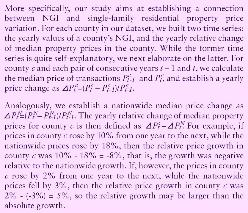
Despite the fact that a lot of research has been done on gentrification at the macroeconomic level, it has not been extensively studied at the microeconomic level using large-scale granular data. This article attempts to correct that.
Gentrification is regarded as one of the main driving forces of the real estate industry: investors look for neighborhoods that start gentrifying, with the intention to invest in them and, ultimately, generate high returns.
This article starts with an examination of how gentrification can be measured at a neighborhood level and utilized to compare between neighborhoods. We then investigate whether gentrification positively affects neighborhood development.
We propose a Normalized Gentrification Index (NGI) of a neighborhood and use it to compare different neighborhoods. In this initial study, we use US counties for neighborhoods, while we plan fine-grained studies in the future. Depending on the underlying data availability, the NGI can be computed at any level of granularity: for US states, counties, metropolitan areas, submarkets, zip codes, census tracts, and so forth.
In this initial study, we chose to focus on the level of counties. We constructed a dataset of 630 US counties for which we had enough data to compute NGI values for each year between 2008 and 2021 and demonstrate their usefulness for real estate investors. We identified a statistical connection between the dynamics of NGI over time and the key performance metric of counties, measured by their residential property prices. We illustrated our findings on two use cases. While we chose residential property prices due to the data abundance, these findings may also be relevant for multifamily, which remains a dominant institutional asset class.
NICHE TRANSFORMATION
In recent years, multifamily investors have experienced a stronger bull market as compared to other asset classes.1 However, as the rising tide has lifted (almost) all boats, a potentially receding tide necessitates a more selective investment strategy.
Just as asset allocation is a primary driver of portfolio returns in a mixed asset class portfolio (e.g., stocks, bonds, etc.),2 selection decisions at the metropolitan statistical area (MSA) level or county level drive the bulk of returns within the real estate investment universe, with individual asset selection relegated to the second place in the return composition hierarchy. Our analysis indicates that—in the majority of cases—a residential property’s price can be predicted within a 20% margin solely based on its county, which validates the importance of county-level selection.
Real estate portfolio management can be enhanced by a proactive, “top-down” market selection approach highlighting locations with potential for above-market return profiles. “Bottom-up” individual investment-level strategies can be supplemented rather than replaced with these analyses. Knowledge of high-potential target counties within the investable universe can ultimately be an alpha enhancer in a competitive investment market.
But there are more than 3,000 counties in the US, so where shall we start?
Our goal is to go beyond trailing signals and momentum-driven strategies and to attempt to create forward-looking signals that may present above-average returns in future years. Specifically, can individual- or family-level wealth inflows predict residential real estate price patterns?
RETHINKING POPULATION DATA
Our primary model in this analysis can be characterized as the gentrification of a neighborhood, which is defined as the net wealth inflow relative to the wealth of the neighborhood. We propose an NGI of a neighborhood and use it to compare different neighborhoods.
The NGI is calculated as the difference between the estimated wealth excess of the in-migration and out-migration of the focal county. Counties with a high NGI have positive wealth inflows, meaning that when we estimate the wealth of in-migrants and out-migrants, there is a net increase. And vice versa for negative NGIs. We consider our NGI as a proxy for gentrification measure.
Obviously, NGI does not fully explain property price changes. In our dataset of 630 US counties, the NGI variation from 2010 to 2020 only weakly correlates with residential price change (r = 0.293), which has a marginally higher correlation compared to a simple demographic indicator such as a population increase estimate (r = 0.177). However, population changes are measured at a very low cadence (typically, once a decade) and cannot reliably be predictive. NGI, in contrast, can be measured quarterly. Moreover, we report a statistical connection between NGI and property price increase, which indicates a predictive power that NGI has on prices. While NGI is not yet fully studied, our first results look promising.
County-level housing supply can often be inelastic, which we assumed would increase prices as new residents bid up the existing real estate inventory. As expected, population growth is more correlated with residential real estate prices in high-barrier-to-entry markets that are characterized by low growth in new housing units.
However, as we analyzed the NGI of these counties based on the bifurcation between high- and low-barrier-to-entry counties, counterintuitively, we saw that the NGI had a stronger relationship with low-barrier-to-entry markets than high-barrier-to-entry markets (if we consider only low-barrier-to-entry counties, the correlation goes up from 0.293 to 0.456).
There are several potential explanations for this dynamic. Firstly, in supply-constrained markets, the utility of adding the wealth dimension to the net population growth may be reduced, because the primary effect will be on adding incremental demand, irrespective of wealth levels. Secondly, elastic supply markets may be lower-cost markets, which are more sensitive to incremental wealth inflows, because the economic effect of this net wealth addition might be more significant throughout the county. To illustrate these dynamics, we have analyzed two counties representing strictly divergent trends: Pinal County, AZ and Cape May County, NJ.
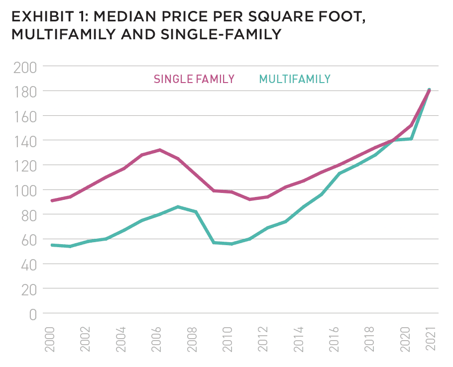
Our empirical study focuses on the statistical connection between NGI and single-family price dynamics, primarily because we have a large number of single-family transactions that ensure statistical signifi cance. We claim that our results are likely to be valid for the multifamily asset class as well. While there are two orders of magnitude fewer multifamily transactions than single-family transactions (at the per-county per-year level), multifamily prices and single family prices highly correlate (r = 0.9). Exhibit 1 illustrates of the similarity of median prices per square foot in the multifamily and single-family markets nationwide.
WHAT IS A NORMALIZED GENTRIFICATION INDEX?
Intuitively, the gentrification of a neighborhood depends on both inbound and outbound migration; namely, a neighborhood is gentrifying if higher-income people are moving into it and/or lower-income people are moving out. The notions of “richer” and “poorer,” for the sake of this article, are relative to the average wealth of the neighborhood’s residents.
Gentrification is cyclic: while richer people are moving in and becoming residents, the average level of wealth of the neighborhood residents rises until it becomes high enough so that people moving in are no longer richer than the average, and then the opposite process of “de-gentrification” starts until the average wealth goes down, for the gentrification to pick up again.
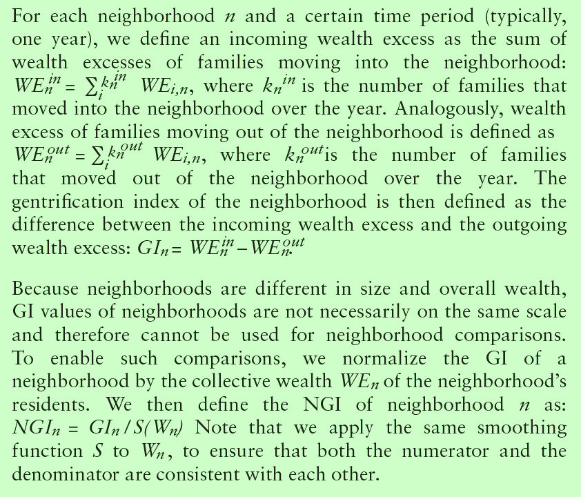
We measure gentrification by utilizing the notion of “wealth excess” of a household i with respect to the average wealth Wn of a household in neighborhood n. We define the wealth excess of household i in neighborhood n as WEi,n = S(Wi–Wn), where Wi is an estimated wealth of i, and S is a smoothing function that levels down extreme differences between Wi and Wn. Smoothing is necessary to take care of edge cases and data issues as explained below. We highlight that WEi,n might be negative if i is poorer than the average in n.
We use a propriety algorithm to estimate household wealth, which bases our estimation on home values, as homeownership is typically the primary source of wealth for a family. For the purposes of this analysis, if we could not obtain the value of a family’s home, we approximate it with an average home value in the same neighborhood.
As mentioned, the NGI of a neighborhood will be positive if many richer families are moving in, and many poorer families are moving out. It will be around zero if few families are moving in and out, or those moving families are of average wealth. The index will be negative if many poorer families are moving in, and many richer families are moving out. Note that if the smoothing function S was not applied, the NGI value might have been primarily influenced by very few wealth excess values WEi,n if they are truly outstanding. For example, if the wealth of a family happens to be estimated at three orders of magnitude compared to the average wealth of a neighborhood’s residents, then this family’s wealth excess would be the dominant factor in the neighborhood’s NGI, which is obviously an undesired outcome.
DATASET
NGI can be defined for “neighborhoods” at any level of granularity, such as MSAs, zip codes, and census tracts. In this work, we analyze NGIs at the coarse level of counties.
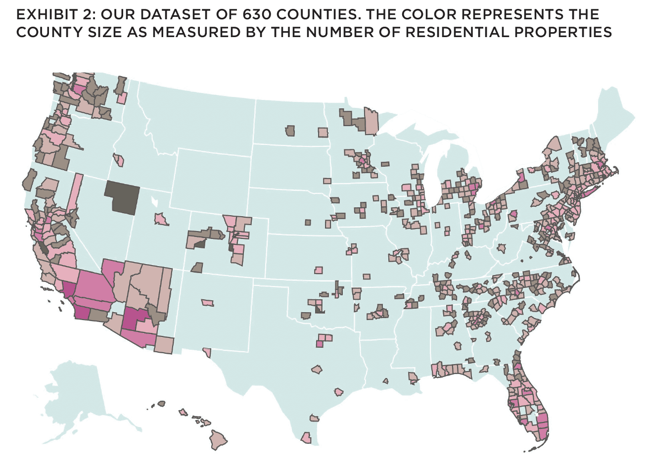
Out of 3,243 US counties and county equivalents, we select only the counties for which we have enough assessed property value data, transaction price data, and relocation data. We also make sure that assessed property values are not too low when averaged over all properties in a county (low average values per square foot might be due to a data artifact) and that property values and transaction prices would be in the same ballpark (very large difference between them would be caused by another data artifact). The selection process resulted in a dataset with 630 counties, covering the majority of the largest US counties that are also attractive destinations for investment capital. Out of the 398 largest US counties reported by the World Population Review,3 334 counties are present in our dataset. Those that are not present are either located in non-disclosure states (so they lack transaction price data) or their data is only partially populated in public data sources. For example, assessed property value data of Cook County, IL (the second largest US county) is populated only from 2017. Exhibit 2 shows our dataset of 630 counties displayed on the map, where the color represents the size of the county in terms of the number of residential properties.
Our relocation dataset consists of 14.4 million relocation records spread over the 2000–21 time period. Each record contains the name of a person, their previous address, their new address, and the year of the relocation. Names of people are not used in this research. The relocation dataset was constructed from public data sources (property sale transactions and property tax records) using a proprietary record-matching algorithm. Each address is associated with the name of the county to which it belongs.
Our relocation dataset is only a subset of all US relocations. However, it does not show a selection bias: on the 630 counties, the Pearson correlation between the number of relocations into a county and the size of the county (measured in the number of residential properties) is high (r = 0.855). The correlation between the number of relocations out of a county and the size of the county is even higher (r = 0.94).
EXLORE THE FULL ISSUE

ALSO IN THIS ISSUE
AFIRE INTERNATIONAL INVESTOR SURVEY: Q1 2023 PULSE REPORT
Gunnar Branson and Benjamin van Loon | AFIRE
VALUATION CHALLENGE: SOLVING THE CRISIS IN COMMERCIAL REAL ESTATE VALUATION
Matt Pomeroy, MAI and Jackie Bowie | Chatham Financial
CONVERSION CALCULATOR: LEGAL OR NOT, A DYNAMIC CITY WILL CONVERT UNUSED OFFICES
Jim Costello | MSCI Real Assets
UNDERWRITING ROADBLOCKS: CAN THE HOSPITALITY MODEL OF UNDERWRITING SAVE OFFICE VALUES?
Joshua Harris, PhD | Lakemont Group & Fordham University
VACANT SPACE: OFFICE-USING JOBS AND DEMAND INCONGRUITY
Stewart Rubin and Dakota Firenze | New York Life Real Estate Investors
HIKING TRAILS: SHOULD INVESTORS CONSIDER ALLOCATIONS TO FLOATING-RATE DEBT?
Dags Chen, CFA | Barings Real Estate
RECESSION PREPPING: HOW VULNERABLE ARE COMMERCIAL MORTGAGE INVESTMENTS
Martha Peyton, PhD | Aegon Asset Management
MEASURING GENTRIFICATION: USING DATA SCIENCE TO PREDICT THE IMPACTS OF GENTRIFICATION
Ron Bekkerman | Cherre + Donal Warde | Tenney 110 + Maxime C. Cohen | McGill University
THE FUTURE IS EUROPEAN: THEMES FROM THE OLD WORLD SHAPING US MARKETS
Brian Klinksiek | LaSalle Investment Management
CULTURE SHOCK: THE CHALLENGE AND IMPORTANCE OF TRANSLATING ESG ACROSS BORDERS
AFIRE ESG Committee
FINE TUNING: GLOBAL REACH AND LOCAL EXPERTISE CAN CREATE UNIFIED REAL ESTATE EXPERIENCES
Mark Zettl | JLL
ACCESSING SUCCES: EXPLORING DIVERSITY TRENDS IN REAL ESTATE TALENT
Zoe Huges | NAREIM
RESCUE CAPITAL: RESPONDING TO THE NEW REAL ESTATE REALITY
Andrew Weiner and Joshua M. R. Becker | Pillsbury
CONVEX CURVES: A REMINDER ON PRICE CONVEXIVITY AND CAP-RATE VOLATILITY
Joseph Pagliari, PhD, CFA, CPA | University of Chicago
IN MEMORIAM: ANDREA MARIE CHEGUT, PhD, MIT
RESULTS
In this paper, we do not attempt to identify the causal effect that the NGI of counties might have on county development. While we leave that for future work, we focus here on measuring correlations, which would indicate statistical connections between NGI and county characteristics.
For each county in our dataset, we computed the Pearson correlation between the two time series, and counted the number of counties for which the correlation was strictly positive (r > 0.5) as well as the number of counties for which it was strictly negative (r < -0.5). We then report on the ratio between those two numbers. We repeat this process for cases when the two time series lag relative to each other, both positively and negatively. A positive lag of 1 means that the NGI time series starts one year earlier than the price change time series, and also ends one year earlier. A negative lag of 1 means that the NGI time series starts one year later than the price change time series and also ends one year later. Lags of -2, 2, and 3 are defined analogously (Exhibit 3).
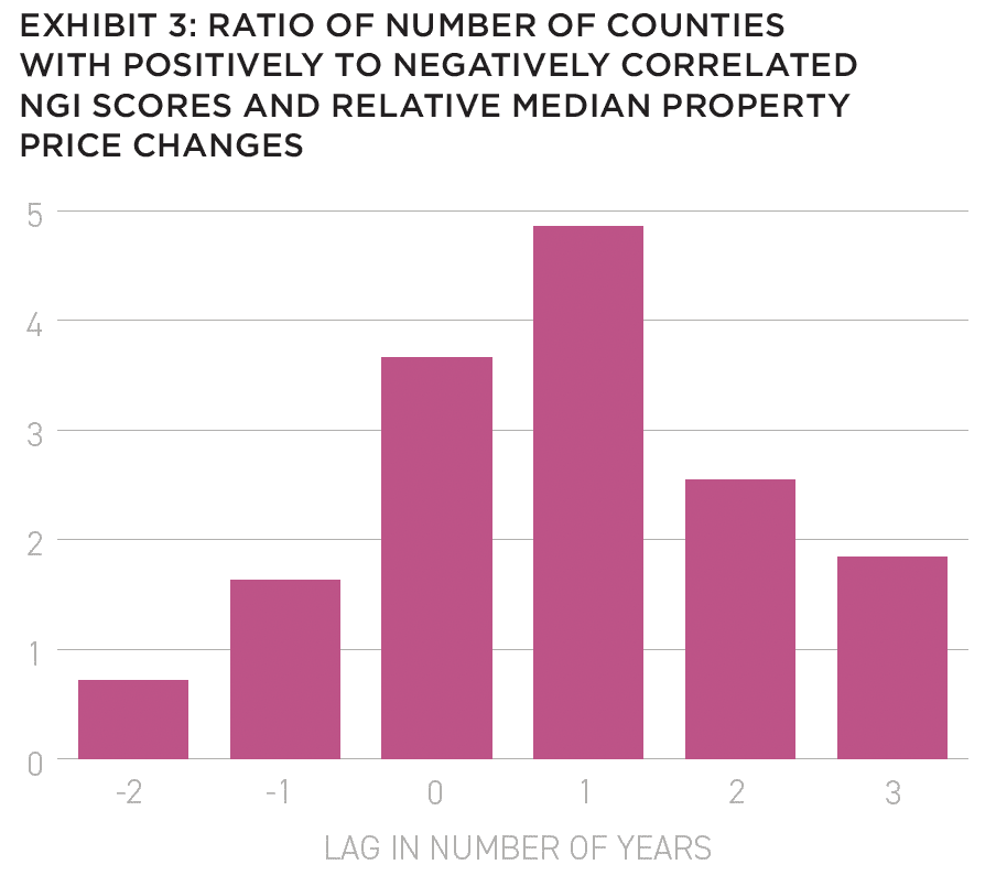
As we can see, for a lag of 0 (i.e., both time series start and end in the same year), there are 3.7 times more strictly positively correlated time series than strictly negatively correlated ones. This implies that property prices fluctuate similarly to the NGI values for 3.7 times more counties than those for which the prices fluctuate differently from the NGI values.
Remarkably, for a lag of 1 (i.e., NGI values precede price changes by one year), this ratio grows to 4.9: property prices follow NGI values almost five times more often than they don’t follow NGI values. The growth of this ratio from 3.7 to 4.9 indicates some predictive power of the NGI.
For a lag of two years, the ratio drops significantly to 2.5, that is, although we can still see more counties in which prices follow NGIs two years later, the number of such counties is not much larger than the number of counties in which prices do not follow NGIs. For a lag of three years, the ratio falls even more, down to 1.8. Remarkably, it is still above 1 (i.e., there are more counties in which prices follow NGIs even three years after).
Negative lags (i.e., price changes precede NGIs by one or two years) show a different picture: while for a lag of -1 there are insignificantly more counties where NGIs follow prices than those where NGIs do not (the ratio is 1.6), for a lag of -2 this ratio drops to 0.7, which means that there are more counties for which NGIs do not follow prices than those for which NGIs do. This implies that property price changes have little to no predictive power over NGI values.
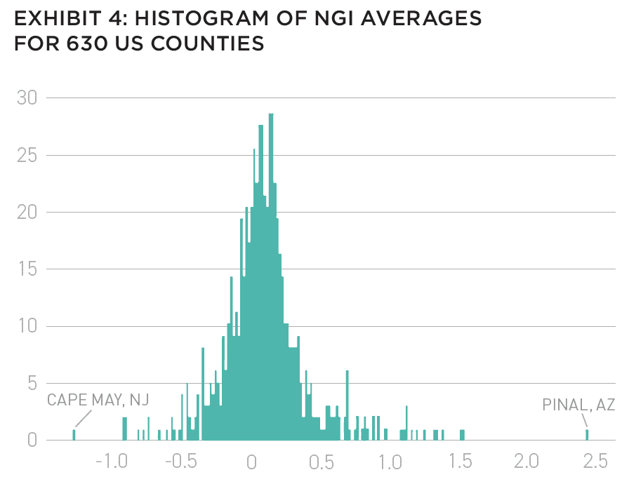
Given the selected 630 counties, the histogram of their NGI values (averaged over the years) is reported below:
As we can see in Exhibit 4, the majority of average NGI values fall around zero (with a mean of 0.09 and a standard deviation of 0.34), while some of the counties are truly outstanding. Specifically, Pinal County, Arizona has exceptionally high NGI values (with an average of 2.4), while Cape May County in New Jersey has very low NGI values (with an average of -1.3).
Yearly NGI values of Pinal County, AZ are shown on the top panel in Exhibit 5. We can see that they are consistently positive, with two peaks in 2009 and 2017. The bottom panel illustrates the relocation numbers, in and out of Pinal County (positive numbers represent inbound traffic, whereas negative numbers correspond to outbound traffic). We show the relocation numbers relative to the inbound relocation in 2008.
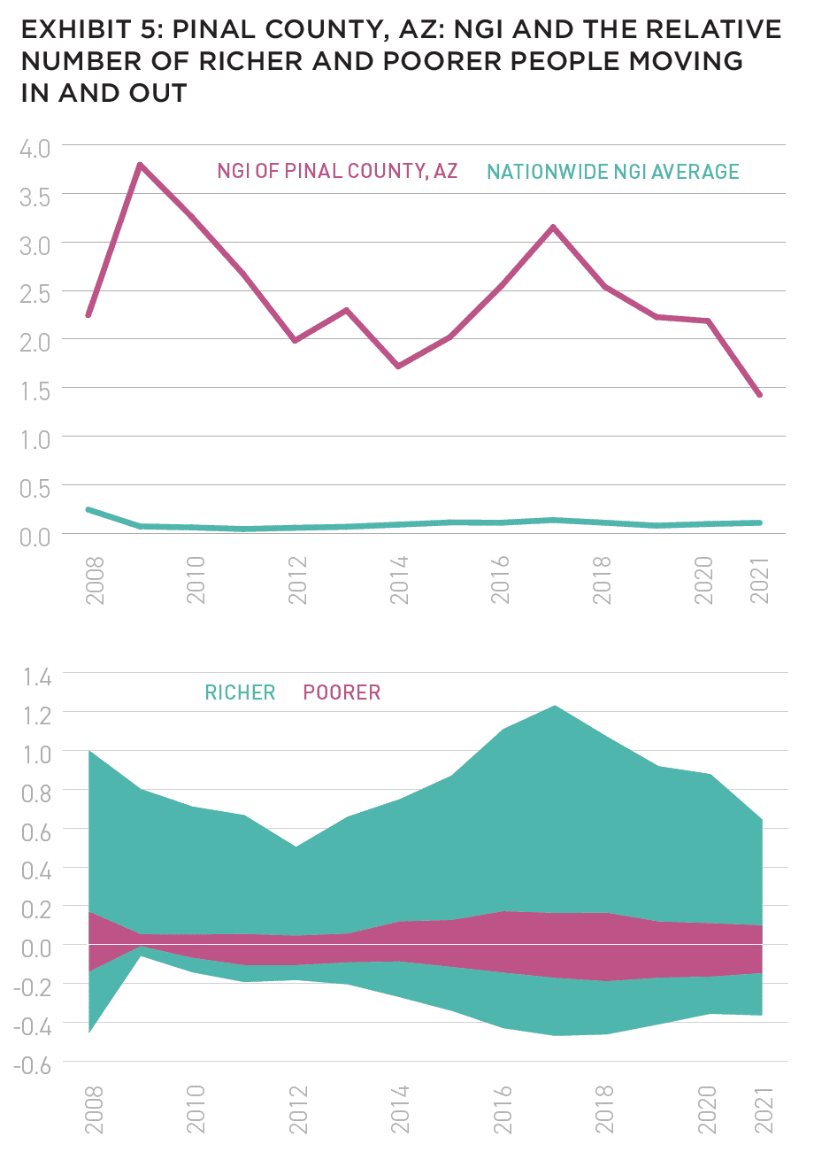
From the bottom panel in Exhibit 5, it is clear that the inbound traffic is substantially stronger relative to the outbound traffic, which is primarily defined by the richer cohort: the number of richer people relocating into Pinal County is significantly greater than the number of richer people relocating out of it. As for the poorer population, the trend is reversed: the number of poorer people relocating into Pinal County is slightly smaller than the number of poorer people relocating out of it. This is consistent with our intuition on the factors that would make NGI values high. The majority of high-end inbound traffic comes from the nearby city of Phoenix, followed by California and (with a substantial gap) by the states of Washington and Colorado. The high-end outbound traffic is mostly within Arizona.
The peak in 2009 is explained by an almost non-existent outbound traffic. The peak in 2017 is associated with a very strong inbound traffic, specifically among the richer population. A certain decline of NGI from 2017 to 2021 is likely caused by an overall decline in relocations. We note, however, that there is no direct connection between the number of relocations and the value of NGI, because NGI takes into account the wealth excess those relocations bring in and out of the county. Specifically, if fewer people move in but they bring more capital, the NGI values may be higher than when more people move in, but they bring less capital.
In terms of residential property prices, we can see a very healthy growth starting from 2011, as shown in Exhibit 6.

While on the nationwide level property prices doubled since 2011, in Pinal County they trebled, and reached the national average pricing in 2021. Note that the NGI time series of Pinal County does not correlate with its property price time series (r = -0.4), however, exceptionally high NGI values suggest a strong gentrification, which is likely to lead to a high appreciation.
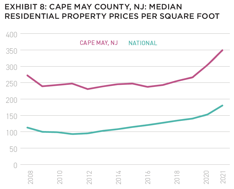
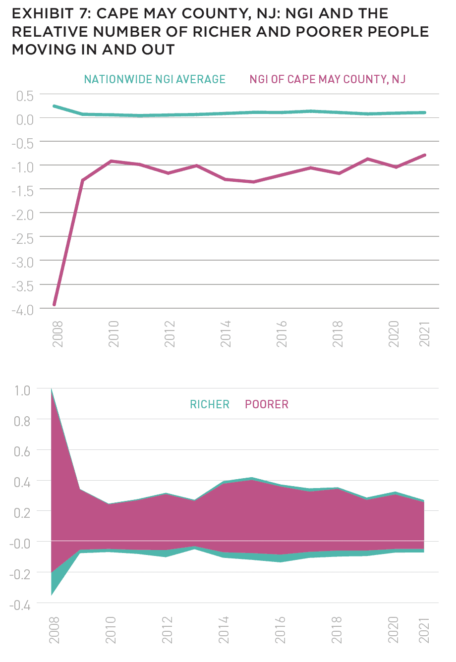
As we could expect, Cape May County, NJ behaves very differently from Pinal County, AZ. Cape May’s NGI values are overly negative (Exhibit 7, upper panel), and this is due to a very strong inbound traffic of people who are less wealthy than Cape May residents (Exhibit 7, bottom panel). Cape May is a luxurious resort community on the Southern coastline of NJ, with home prices being significantly above the national medians (Exhibit 8). With the majority of inbound traffic coming from the nearby counties of Pennsylvania and New Jersey, Cape May’s wealth is just greater than that of most of its neighbors and, thus, the county cannot be further gentrified.
The lack of gentrification ultimately affects the home price dynamics. Overall, the prices rise in Cape May slower than the nationwide average. Nevertheless, they kept relatively unchanged during the 2009-2011 recession (when nationwide prices slipped), and then rose faster in 2020 during the pandemic. Their counter-cyclical behavior is in compliance with the resort, get-away nature of the county.
THE FUTURE OF GENTRIFICATION RESEARCH
Our proposed NGI provides a useful tool for real estate investment managers to optimize their investment decisions. National population and income levels can obfuscate significant variation between counties within the US, which offer abundant opportunities to identify and take advantage of county-level trends.
Just as prudent multifamily owners underwrite the creditworthiness of a potential renter (as opposed to immediately accepting), migration patterns can be subject to comparable financial underwriting of households who change counties. Such an analysis can impact our understanding of the materiality of each move and its potential influence on the real estate market of a given county.
Future research on this topic may include a deeper analysis of explanations for why the NGI seems to have predictive power, and the variation of such predictions across different market characteristics, such as differences between in-state and out-of-state moves, and comparing NGI values with real estate pricing forecasts.
—
ABOUT THE AUTHORS
Ron Bekkerman is a Strategic Advisor and a former Chief Technology Officer of Cherre, a leading real estate data platform. Donal Warde is an Entrepreneur in Residence at Tenney 110, a PropTech venture studio, and worked in private equity real estate for several years. Maxime C. Cohen is the Scale AI Chair Professor of Retail and Operations Management and Director of Research at McGill University.
NOTES
1. CBRE. “Steady Investment Activity Shows Commercial Real Estate Resilience,” CBRE Insights, accessed April 24, 2023, cbre.com/insights/viewpoints/steadyinvestment-activity-shows-commercial-real-estate-resilience.
2. Brinson, Gary P., L. Randolph Hood, and Gilbert L. Beebower. “Determinants of Portfolio Performance.” Financial Analysts Journal 51, no. 1 (January/February 1995): 133-138. cfainstitute.org/en/research/financial-analysts-journal/1995/determinants-of-portfolio-performance.
3. World Population Review. “List of Counties in the United States.” Accessed April 24, 2023. worldpopulationreview.com/us-counties.
—